Spectral Signature Analysis

Goal

Background: The goal of this lab was to gain experience on the measurement and interpretation of spectral reflectance.

Methods

In order to collect the necessary data for this assessment an image of Eau Claire was brought into Erdas. The "Home" tab was selected, followed by "Drawing" and then the "Polygon" tool was selected in order to create various Areas of Interests (AOIs). After the AOI was selected, the "Raster" tab was chosen, followed by "Signature Editor" and then "Signature Editor". This opened the "Signature Editor" window, where the option to create a new AOI was selected. This brought in the AOI that was just created using the polygon tool. After each AOI was brought in, the name was changed to its respective feature. The twelve features examined were: 1) Standing Water; 2) Moving Water; 3) Vegetation; 4) Riparian Vegetation; 5) Crops; 6) Urban Grass; 7) Dry Soil (uncultivated); 8) Wet Soil (uncultivated); 9) Rock; 10) Asphalt Highway; 11) Airport Runway; 12) Concrete Surface (Parking Lot).

After the AOI was brought into Signature Editor, the "Display Mean Plot Window" option was selected, which allowed for the observance of the Spectral Signature. Below are Figures 1-13, which show the various spectral signatures of the twelve features and one figure showing all of them on the same plot.

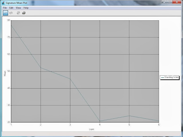Figure 1: This plot shows the spectral signature for Standing Water. The most reflectance is seen in the blue and green bands is the least reflectance are seen in the red and infrared bands.

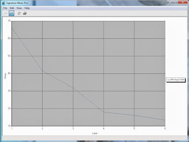Figure 2: This plot shows the spectral signature for Moving Water. The most reflectance is seen in the blue band and the least reflectance is seen in the infrared band.

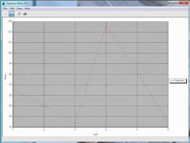Figure 3: This plot shows the spectral signature for Vegetation. The most reflectance is seen in the red and infrared bands and the least reflectance is seen in the blue and green bands.

Figure 4: This plot shows the spectral signature for Riparian Vegetation. The most reflectance is seen in the red and infrared bands and the least reflectance is seen in the blue and green bands.

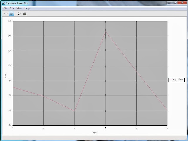Figure 5: This plot shows the spectral signature for Crops. The most reflectance is seen in the red and infrared bands and the least reflectance is seen in the blue and green bands.

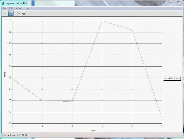Figure 6: This plot shows the spectral signature for Urban Grass. The most reflectance is seen in the red and infrared bands and the least reflectance is seen in the blue and green bands. The background was changed for this plot to make the spectral signature line more visible.

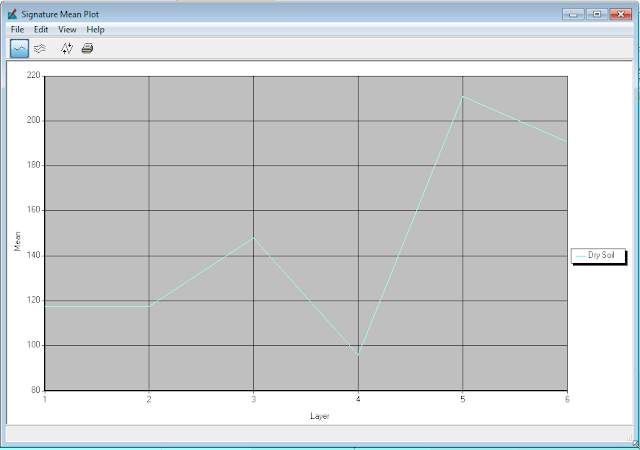Figure 7: This plot shows the spectral signature for Dry Soil. The most reflectance is seen in the red and mid infrared bands and the least reflectance is seen in the blue band.

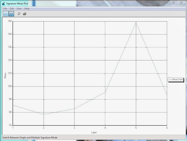Figure 8: This plot shows the spectral signature for Moist Soil. The most reflectance is seen in the red and infrared bands and the least reflectance is seen in the blue and green bands. The background was changed for this plot to make the spectral signature line more visible.

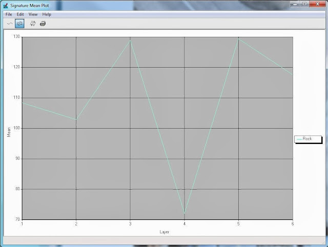Figure 9: This plot shows the spectral signature for Rock. The most reflectance is seen in the green and infrared bands and the least reflectance is seen in the red band. 

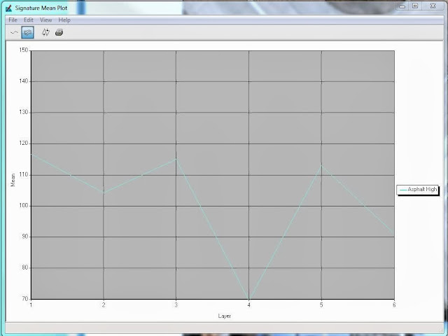Figure 10: This plot shows the spectral signature for Asphalt Highway. The most reflectance is seen in the green and infrared bands and the least reflectance is seen in the red band. 

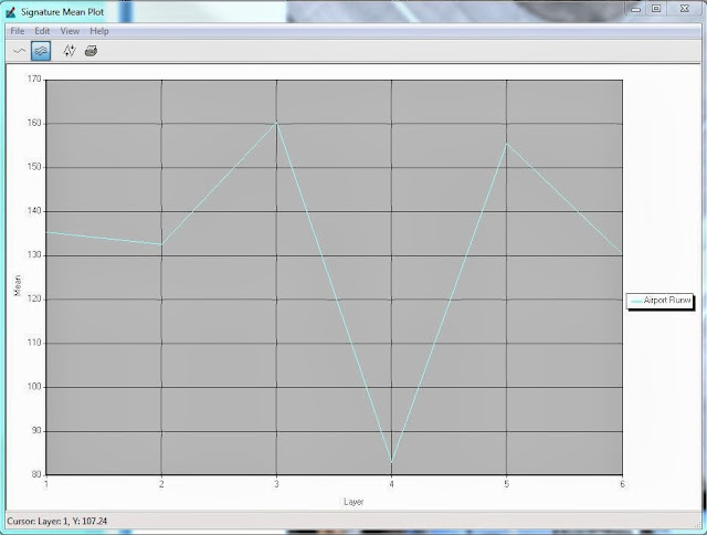Figure 11: This plot shows the spectral signature for Airport Runway. The most reflectance is seen in the green and infrared bands and the least reflectance is seen in the red band. 

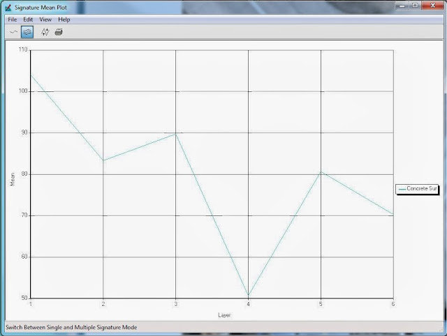Figure 12: This plot shows the spectral signature for Concrete Surface. The most reflectance is seen in the blue, green, and infrared bands and the least reflectance is seen in the red band. 

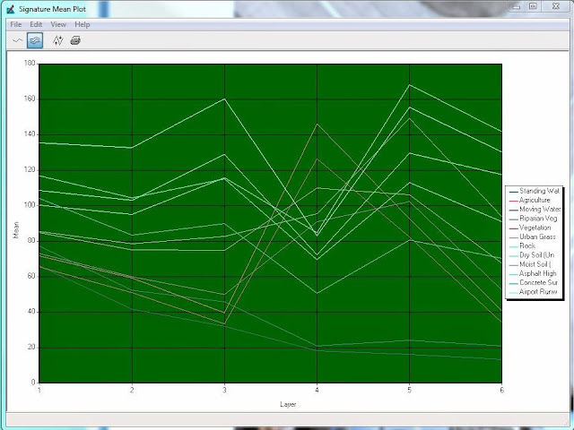Figure 13: This shows all of the spectral signatures on the same plot. Trends can be seen between water surfaces, vegetated surfaces, and non-vegetated surfaces in relation to their spectral signatures.