Spectral Signature Analysis

Goal

Background: The goal of this lab was to gain experience on the measurement and interpretation of spectral reflectance.

Methods

In order to collect the necessary data for this assessment an image of Eau Claire was brought into Erdas. The "Home" tab was selected, followed by "Drawing" and then the "Polygon" tool was selected in order to create various Areas of Interests (AOIs). After the AOI was selected, the "Raster" tab was chosen, followed by "Signature Editor" and then "Signature Editor". This opened the "Signature Editor" window, where the option to create a new AOI was selected. This brought in the AOI that was just created using the polygon tool. After each AOI was brought in, the name was changed to its respective feature. The twelve features examined were: 1) Standing Water; 2) Moving Water; 3) Vegetation; 4) Riparian Vegetation; 5) Crops; 6) Urban Grass; 7) Dry Soil (uncultivated); 8) Wet Soil (uncultivated); 9) Rock; 10) Asphalt Highway; 11) Airport Runway; 12) Concrete Surface (Parking Lot).

After the AOI was brought into Signature Editor, the "Display Mean Plot Window" option was selected, which allowed for the observance of the Spectral Signature. Below are Figures 1-13, which show the various spectral signatures of the twelve features and one figure showing all of them on the same plot.

Figure 1: This plot shows the spectral signature for Standing Water. The most reflectance is seen in the blue and green bands is the least reflectance are seen in the red and infrared bands.

Figure 2: This plot shows the spectral signature for Moving Water. The most reflectance is seen in the blue band and the least reflectance is seen in the infrared band.

Figure 3: This plot shows the spectral signature for Vegetation. The most reflectance is seen in the red and infrared bands and the least reflectance is seen in the blue and green bands.

Figure 4: This plot shows the spectral signature for Riparian Vegetation. The most reflectance is seen in the red and infrared bands and the least reflectance is seen in the blue and green bands.

Figure 5: This plot shows the spectral signature for Crops. The most reflectance is seen in the red and infrared bands and the least reflectance is seen in the blue and green bands.

Figure 6: This plot shows the spectral signature for Urban Grass. The most reflectance is seen in the red and infrared bands and the least reflectance is seen in the blue and green bands. The background was changed for this plot to make the spectral signature line more visible.

Figure 7: This plot shows the spectral signature for Dry Soil. The most reflectance is seen in the red and mid infrared bands and the least reflectance is seen in the blue band.

Figure 8: This plot shows the spectral signature for Moist Soil. The most reflectance is seen in the red and infrared bands and the least reflectance is seen in the blue and green bands. The background was changed for this plot to make the spectral signature line more visible.

Figure 9: This plot shows the spectral signature for Rock. The most reflectance is seen in the green and infrared bands and the least reflectance is seen in the red band. 

Figure 10: This plot shows the spectral signature for Asphalt Highway. The most reflectance is seen in the green and infrared bands and the least reflectance is seen in the red band. 

Figure 11: This plot shows the spectral signature for Airport Runway. The most reflectance is seen in the green and infrared bands and the least reflectance is seen in the red band. 

Figure 12: This plot shows the spectral signature for Concrete Surface. The most reflectance is seen in the blue, green, and infrared bands and the least reflectance is seen in the red band. 

Figure 13: This shows all of the spectral signatures on the same plot. Trends can be seen between water surfaces, vegetated surfaces, and non-vegetated surfaces in relation to their spectral signatures.

Photogrammetry

Goal

Background: The goal of this lab was to develop skills to perform photogrammetric tasks on aerial photographs and satellite images.

Methods

Scales, Measurements, and Relief Displacement:

Section 1: Determining scale is a very essential part of interpreting distance on maps. For the first portion of this assignment, real world points and their distances were provided and the scale had to be determined from them. The distance from point-to-point was measured using a ruler and then the was converted to a relative scale number by multiplying the real world distance, by 12 in order to convert it to inches, then it was divided by the number of inches measured by the ruler. The resulting number provides a relative number, or the scale, of the map (Figure 1). 

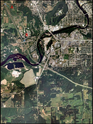Figure 1: Fore this method, the distance from Point A to
Point B was measured wit ha ruler and, using the given
real world distance, a scale was determined for this image.

Scale can also be determined by using the focal length lens of the camera, the altitude of the lens, and the elevation of the object above sea level.

Section 2: Another way to determine the area of a given feature on Erdas is to use the "Measure" tool. This tool is found under the "Home" tab and allows the analyst to measure various aspects of area. The polygon tool was selected for use and a lagoon to the west-southwest of Eau Claire was digitized. This was used to determine the area in hectares and acres, as well as the perimeter in meters and miles (Figure 2). 

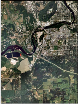Figure 2: This shows the lagoon, denoted by the X, that
was digitized in order to determine area in hectare and
acre, and perimeter in meters and miles.

Section 3: Determining relief displacement allows the analyst to determine how far an object is from their true planimetric location on the ground through use of aerial photographs. The scale of the image was given as was the camera height above the datum. The height of the smokestack was measured and the scale was used to convert it to the smokestack's approximate height. Then, the distance from the top of the smokestack and the principal point was measured and converted to an approximate real-world distance. The numbers were plugged into the relief displacement equation and the approximate height was determined (Figure 3).

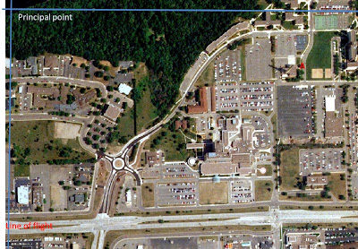Figure 3: The smokestack and Point X was used to determine relief
displacement of the image. The principal point is located in the upper
left corner. The line of flight is denoted by the blue line.

Stereoscopy:

In order to allow for three-dimensional viewing on an image, which is what stereoscopy allows, multiple images were brought in for this exercise. The "Terrain" tab was selected, followed by "Anaglyph" in order to open the "Anaglyph Generation" window. The correct input and output images were determined, the vertical exaggeration of the image was increased to (2), and the model was run (Figure 4). 

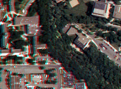Figure 4: In order to properly see the resulting image, polaroid glasses were
worn, which allowed the analyst to see the image in a three-dimensional way.

Orthorectification:

Section 1: The final portion of this lab allows the simultaneous rectification of positional and elevation errors of multiple images. To begin the process of orthorectification, Lecia Photogrammetric Suite (LPS) was opened through Erdas. This program is used for a variety of purposes, one being the orthorectification of images collected by various sensors. A new block file was created and the "Model Setup" window was opened. The correct geometric model category was selected, the correct projection was applied, and the model was prepared for orthorectification. 

Section 2: An image was brought in and "Show and Edit Frame Properties" was selected, followed by "Edit", then "OK" twice. This process specifies the correct sensor that the image is using.

Section 3: Now the main process of recording ground control points was carried out. The GCP icon was selected and "Classic Point Measurement Tool" was chosen as the method. "Reset Horizontal Reference Source" was selected, which opens the GCP Reference Source dialog. "Image Layer" was checked, "OK" was selected, and "Use Viewer As Reference" was selected. The GCPs were then collected in much the same manner as they had in the previous labs. Points were added, the GCP was selected, and the corresponding GCP was selected on the referencing image. After the second point, "Automatic (x,y) Drive" was selected, which allows LPS to approximate where the GCP is on the other image to allow for quicker GCP collection. This was done for nine ground control points. The points were then saved and the last two points were ready to be added. Again, the "Reset Horizontal Reference Source" icon was selected, a new image was brought in, and the last two points were collected. 

Now that the Horizontal Reference Source was set, the Vertical Reference Source needed to be set as well. The "Reset Vertical Reference Source" icon was selected and a Digital Elevation Model image was brought in to supply elevation data. The "Update Z Values on Selected Points" icon was selected and all the Z values, (elevation data) was updated. 

Section 4: The "Type" column was selected and "Formula" was opened in order to set the "Type". In this case the type was set to "Full" and the change was applied. This process was carried out for "Usage" and the usage was set to "Control". The data was saved and the point measurement tool was closed. Next, a second image was brought in. The same work flow was carried out to prepare this image as had been done for the previous image. The GCPs for this image were added as instructed by the guidelines, as portions collected on the previous image were not present for this image (Figure 5). 

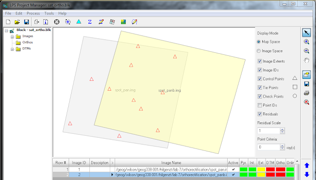Figure 5: This shows the status of orthorectification, thus far. The image is still somewhat tilted, as it has not been fully
rectified yet.

Section 5: "Automatic Tie Point Generation Properties" was selected, opening up a dialog. The necessary characteristics were input, the "Intended Number of Points/Images" was set to forty, and the process was run. Given the data previously collected, this step accurately places even more GCPs and pins the image down even more accurately. This step allows for triangulation of the various components. "Edit" then "Triangulation Properties" was selected to open a dialog. The necessary characteristics were input and a report for the data was generated.

This finally prepared the data to be resampled.  "Start Ortho Resampling Process" was selected and the correct characteristics were input. Bilinear Interpolation was the resampling method used for this process. After all the settings were specified, the model was run and the orthorectified image was produced. 

Section 6: After orthorectification, the images match up properly and are able to be compared (Figure 6). The images are brought into the same viewer and examined to ensure that the various features match (Figure 7 and Figure 8).

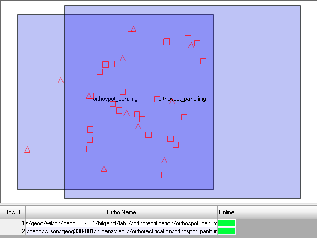Figure 6: After the orthorectification process was complete, the image is rectified to the image above. This shows that the image is properly rectified and is not off improperly referenced.

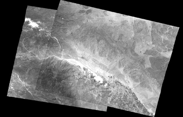Figure 7: This image is the result of the orthorectification process. After properly analyzing and assigning values to the images, they blend together very accurately.

Figure 8: This zoomed in view of the orthorectified image
shows that, while there are very small details that may not
match up perfectly, the orthorectification process leads to
a very accurate image mosaic.

Results

This lab provided an extremely in depth look at photogrammetric processes. An understanding was gained that focused on understanding how scales were formulated for aerial imagery, how stereoscopy and stereograms were created in order to show three-dimensional models, and how multiple photographs can be seamlessly mosaicked through orthorectification.